Seigniorage, Tobin tax, fiat money, gold and Bitcoin

It is obvious that fiat money leads to seigniorage income for the sovereign, but one would imagine that a decentralized open source money like Bitcoin (see my blog post earlier this month) would not allow anybody to earn seignorage income. When one examines the Bitcoin design, we find that it allows those with enough computing power to extract two forms of seigniorage income:

1. In the early years of Bitcoin, computing power allows the mining of new bitcoins. This is pure seigniorage.
2. When most of the coins have been mined, computing power can be used to charge transaction fees on every bitcoin transaction. This is also seigniorage income in the form of an all encompassing Tobin tax beyond the wildest dreams of the proponents of that tax.

Is this a design flaw or is it a necessary feature? After careful consideration, I think it is necessary. A monetary system can be sustained only if there are people with the incentive to invest in the maintenance of the system. In the case of fiat money, the sovereign expends considerable effort in preventing counterfeiting. One might think that commodity money like gold does not require such effort. But the historical evidence suggests otherwise:

1. After the collapse of the Roman empire, “within a generation, by about A.D. 435, coin ceased to be used [in Britain] as a medium of exchange … although many survived as jewellery, or were used for gifts or for compensation.” (Christine Desan, “Coin Reconsidered: The Political Alchemy of Commodity Money”, quoting Peter Spufford.) With nobody having enough seigniorage income to try and maintain the system, commodity money was simply re-purposed to non monetary uses, and Britain relapsed into a barter economy.
2. Christine Desan also points out that a monetary system based on silver was reestablished centuries later by sovereigns who extracted seignorage income by charging a 5-10% spread between the mint and melting points of the metal.
3. On the other hand, Luther and White have several papers showing that after the collapse of the Somalian government, the old currency continued to circulate and local warlords maintained the money supply by counterfeiting the old currency notes to earn seigniorage income.

All this suggests that any form of money (whether fiat, commodity or a decentralized open source money like Bitcoin) needs some form of seigniorage to sustain it.
1

Interest rate modelling at the zero lower bound

A long time ago, before the Libor Market Model came to dominate interest rate modelling, a lot of attention was paid to how interest rate volatility depended on the level of interest rates. If rate are moving up and down by 0.5% around a level of 3%, how much movement is to be expected when the level changes to 6%? One school of thought argued that rates would continue to fluctuate ±0.5%; this very conveniently allows the modeller to assume that rates follow the normal distribution. An opposing school argued that a fluctuation of ±0.5% around a level of 3% was actually a fluctuation of ¹⁄₆ of the level. Therefore when the level shifts to 6%, the fluctuation would be ±1% to preserve the same proportionality of ¹⁄₆ of the level. This was also convenient as modellers could assume that interest rates are log-normally distributed.

It was also possible to take a middle ground – the celebrated square root model related the fluctuations to the square root of the level. A doubling of the level from 3% to 6% would cause the fluctuation to rise by a factor of √2 from 0.5% to 0.71%. People generalized this even further by assuming that the fluctuations scaled as (level)^λ where λ=0 gives the normal model, λ=1 leads to the log-normal, and λ=0.5 yields the square root model. Of course, there is no need to restrict oneself to just one of these three magic values. The natural thing for any statistician to do is to estimate λ from the data using standard maximum likelihood or other methods. Long ago, I did do such estimations for Indian interest rates.

The Libor Market Model killed this cottage industry. It was most natural to assume log normal distributions for the interest rates and then let the option implied volatility smile deal with departures from this distributional assumption. And there matters rested until the problem resurfaced when interest rates were driven down to zero after the global financial crisis. The difficulty is that zero is an inaccessible boundary point for a log normal process. A log normal process (geometric Brownian motion) can not reach zero (in any finite time) starting from any positive rate, and if you somehow started it out from zero, it could never leave zero (because the volatility becomes zero).

The regulatory push to mandate central clearing for OTC derivatives has turned this esoteric modelling issue into an important policy concern because central clearing counterparties (CCPs) have to set margins for a variety of interest rate derivatives where the modelling of volatility becomes a first order issue. A variety of different approaches are being taken. The OTCSpace blog links to a couple of practitioner oriented discussions on this subject (here and here). Among the solutions being proposed are the following:

Shift to a normal model

This would eliminate under margining at zero interest rates, but potentially create severe under margining at high rates.

Combine normal and log-normal fluctuations

The idea is that there are two sources of fluctuations in interest rates – one behaves in a “normal” and the other in a “log-normal” manner. This may be intractable for valuation purposes, but might be acceptable for risk modelling since it solves the under margining problem at both ends of the interest rate spectrum.

Interest rate plus a small constant is log normal

For example, assume that the fluctuations in interest are proportional to the level of rates +1%.

As an aside, I believe that the zero lower bound is actually a bound not on the interest rate, but on the contango on money. In other words, the zero lower bound is simply the proposition that money (being the unit of account itself) can neither be in contango nor in backwardation. The standard cost of carry model for futures pricing tells us that the contango on money is equal to the risk free interest rate PLUS the storage cost of money MINUS the convenience yield. It is this contango that is constrained to be zero.

If the convenience yield of money is larger than the storage costs (as it usually is in normal times), the contango is zero when the interest rate is positive. In an era of unlimited monetary easing, the convenience yield of money can become very small and the zero contango implies a slightly negative interest rate since the storage cost is not zero. For physical currency, the storage cost is high because of the need to guard against theft. For insured bank deposits, the bank needs to recoup deposit insurance in some form through various fees. Of course, uninsured bank deposits are not money – they are simply a form of haircut prone debt (think Cyprus). Actually, Cyprus makes one sceptical about whether even insured bank deposits are money.

Bitcoin, negative interest rates and the future of money

I believe that everybody who is interested in money should study the digital currency Bitcoin very carefully because monetary innovations can have long lasting consequences even when they fail miserably:

1. China’s experiments with paper money ended in inflationary disaster (as almost all fiat money appear to do), but it succeeded in replacing China’s long standing bronze coin standard with a silver unit of account (see for example, Richard von Glahn (2010), “Monies of Account and Monetary Transition in China, Twelfth to Fourteenth Centuries”, Journal of the Economic and Social History of the Orient, 53(3), 463-505)
2. Johan Palmstruch who brought paper money to Europe and founded the world’s first central bank (the Sveriges Riksbank of Sweden) was sentenced to death. Though he was reprieved, he still lost everything and ended up in jail.

There is little doubt in my mind that digital currencies represent a vast technical and conceptual advance over the currencies in existence today. This would remain true even if Bitcoin implodes in a collapsing bubble or is destroyed by technical flaws in its design or implementation.

Nemo at self-evident.org has an excellent ten part series providing a gentle introduction to all the mathematics that one needs to understand how Bitcoin works. This is a good starting point for somebody wanting to go on to Satoshi Nakamoto’s seminal paper introducing the idea of Bitcoin.

From a finance point of view, what is most interesting about Bitcoin is that it is perhaps the first currency to be designed with a strong deflationary bias. There is an upper limit on the number of bitcoins that can ever be created – even lost bitcoins cannot be replaced unlike normal central banks that replace worn out notes with newly printed ones. In paper currencies, if I lose a currency note, somebody else probably finds it, and so the note remains in circulation. By contrast, Bitcoin is so designed that if the owner loses a bitcoin, the “finder” cannot use it, and so the lost bitcoin ceases to exist for all practical purposes. (If you are puzzled by the apparently inconsistent capitalization of bitcoin/Bitcoin in this paragraph, you may want to read this).

While most fiat currencies end up printing notes in higher and higher denominations to combat inflation, Bitcoin is designed to combat deflation by using smaller and smaller denominations like milli bitcoins and micro bitcoins all the way down to the smallest unit named the Satoshi which is equivalent to 10 nano bitcoins. As a result, the zero interest rate lower bound could be an even more serious problem for Bitcoin than for existing currencies.

One theoretical possibility is that the deflation overshoots significantly so that the currency can experience a mild inflation from that point onward somewhat on the lines of the Dornbusch overshooting model. But for that to work on a sustained basis, there would need to be periodic bouts of intense episodic deflation. The sharp appreciation of the bitcoin in the last few weeks in response to the Cyprus crisis suggests one way in which this could happen, but that would be a nightmare to model.

Option pricing with bimodal distributions

Jack Schwager’s book Hedge Fund Market Wizards has a chapter on James Mai of Cornwall Capital in which Mai talks about seeking opportunities in mispriced options. Many of us know about Mai from Michael Lewis’ Big Short which described how Mai made money by betting against subprime securities. But in the Schwager book, Mai talks mainly about options. Specifically, at page 232, Mai discusses opportunities “where the market assigned normal probability distributions to situations that clearly had bimodal outcomes”.

At first reading, I thought that Mai was simply talking about fat tails and the true volatility being higher than the option implied volatility. But on closer reading, this does not appear to be the case. In another section of the interview, Mai talks about the market under estimating the volatility of the distribution, while at another point, he describes the market making mistakes in the mean of the option implied distribution. So it does appear that Mai is distinguishing between errors in the mean, the volatility and the shape of the distribution.

This set me thinking about whether the bimodality of the distribution would make a big difference if the market assumes a (log) normal distribution with the correct mean and variance. Bimodality is very different from fat tails. In fact, if the distribution around each of the two modes is tight, then the tails are actually very thin. The departure from normality is actually a hollowing out of the middle of the distribution. For example, one may believe that a stock would either go to near zero (bankruptcy) or would double (if the risk of bankruptcy is eliminated) – the probability that the stock would remain close to the current level may be thought to be quite small. Mai himself discusses such an example.

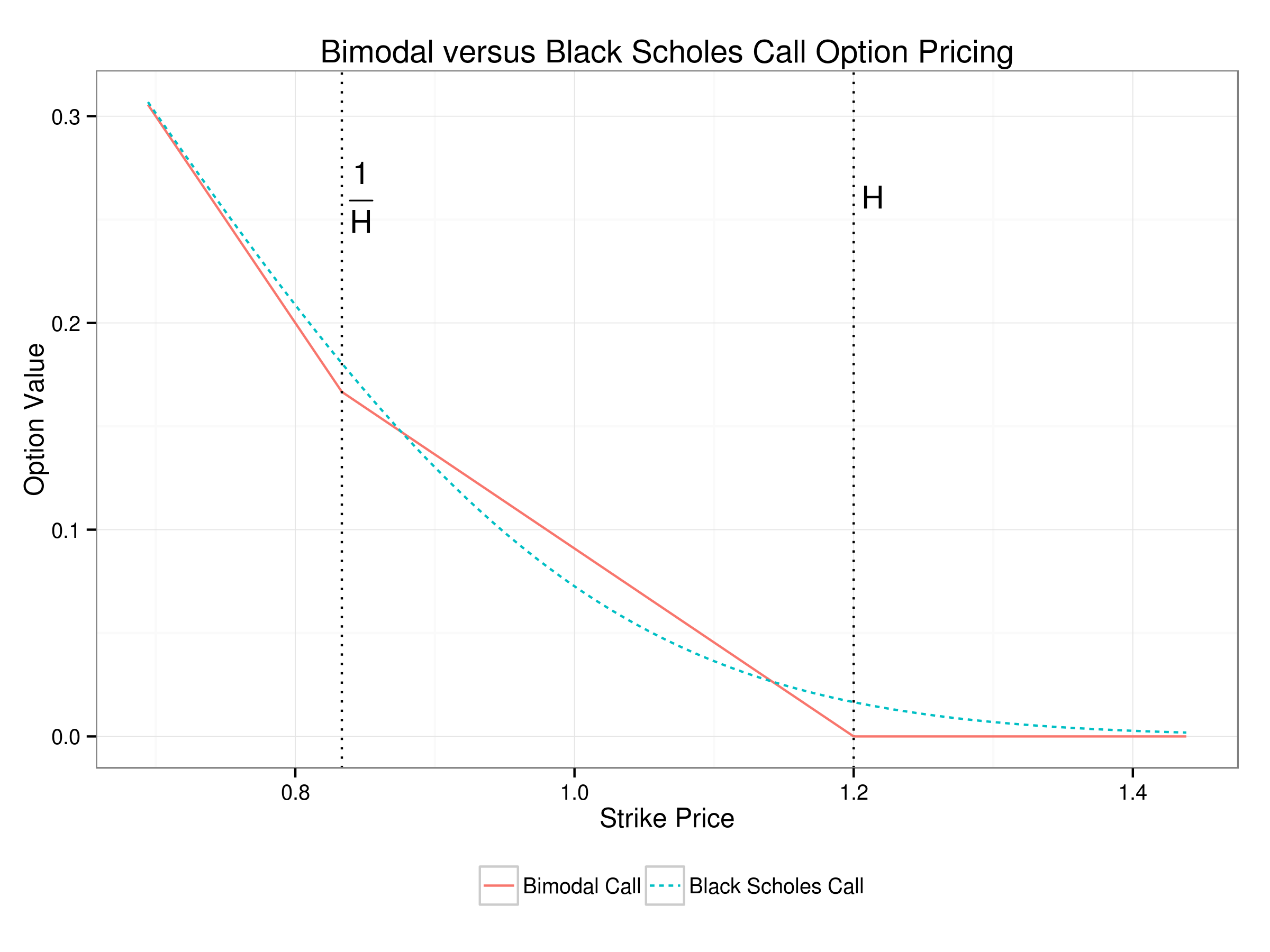
To understand the phenomenon, let us take an extreme case of bimodality where there are actually only two outcomes. For simplicity, I assume that the risk free rate is zero. To facilitate comparison with the log normal distribution, I assume that the distribution of log asset prices is symmetric. If the current asset price is equal to 1, then by log symmetry, the two outcomes must be H and ¹⁄_H. Since the two possible outcomes of the log price are ± ln H, the volatility is ln H assuming that the option maturity is 1. The risk neutral probabilities of the two outcomes (p and 1 − p) are easy to compute. Since the risk free rate is zero, p H + (1 − p) ¹⁄_H = 1 implying that p = 1 ⁄ (1 + H) and 1 − p = H ⁄ (1 + H). (Unless H is quite large, these probabilities are not very far from ¹⁄₂).

With all these computations in place, it is straightforward to compare the true bimodal option price with that obtained by the Black Scholes formula using the correct volatility. The plot below is for H = 1.2.

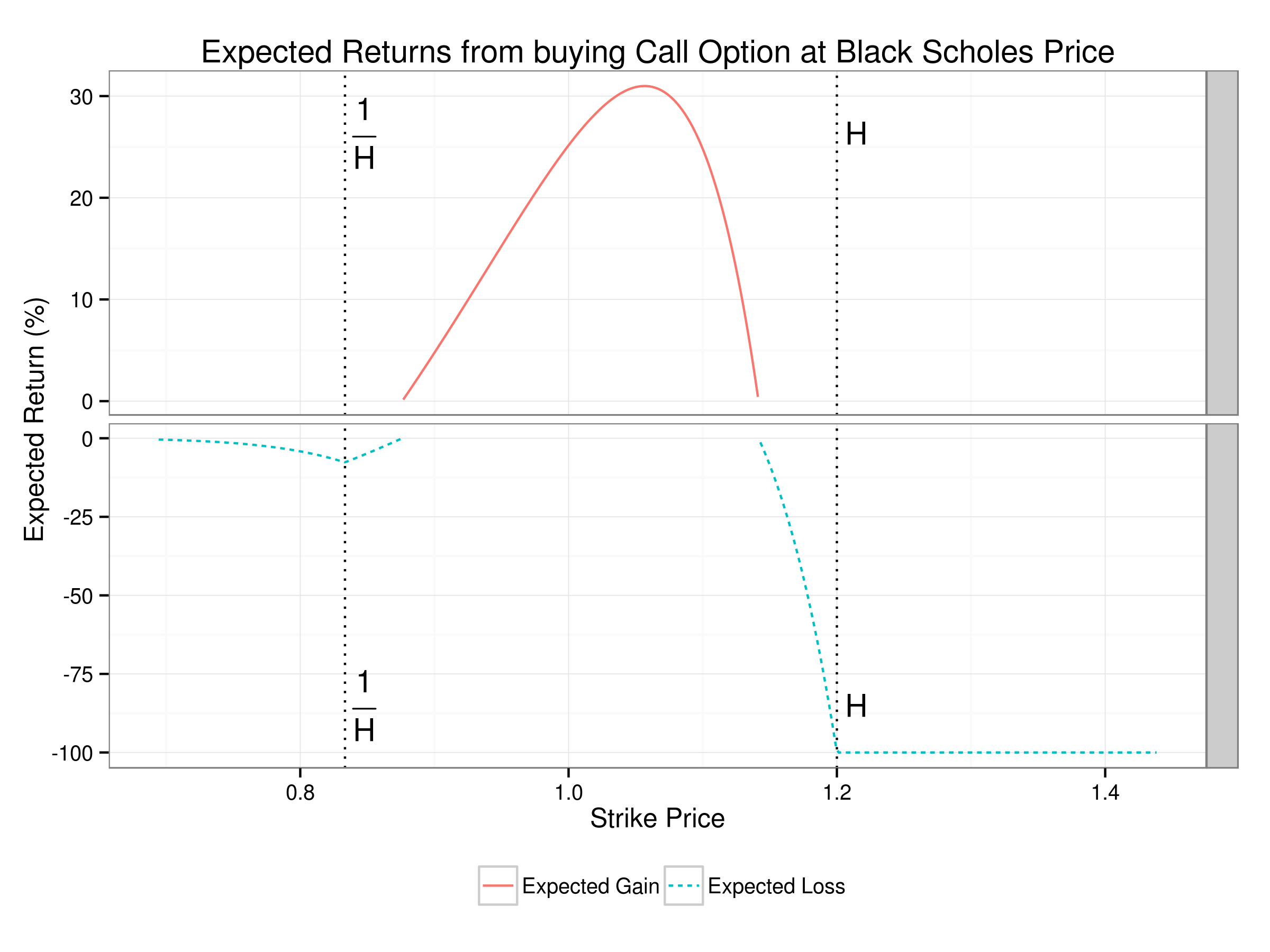
It might appear that the impact of the bimodal distribution is quite small. However, the important question is what is the expected return from buying an option at the wrong (Black Scholes) price in the market and holding it to maturity. The plot below shows that the best strategy is to buy an option with a strike about 6% out of the money. This earns a return of almost 31% (there is a 45% chance of earning a return of 188% and a 55% chance of losing 100%).

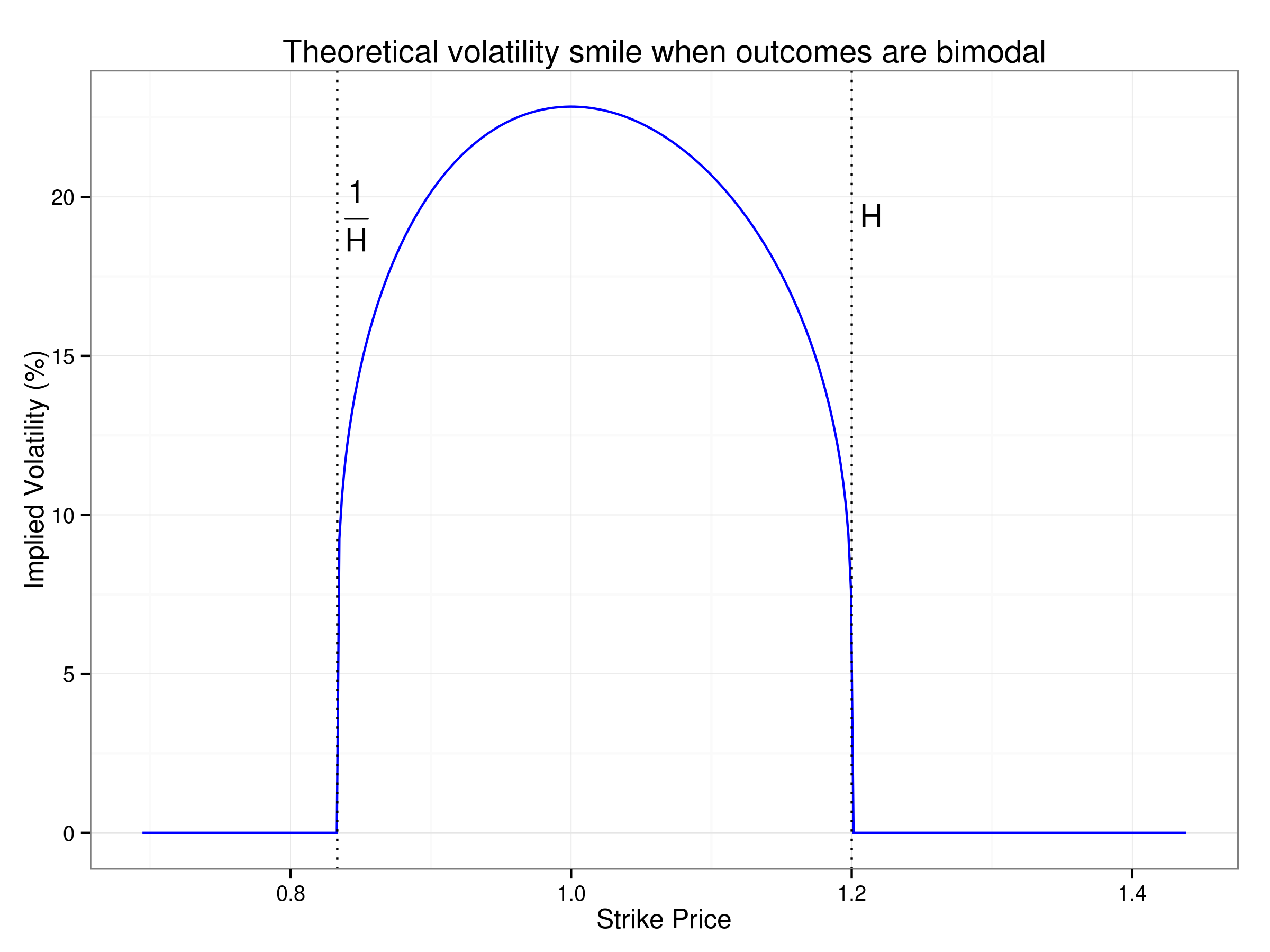
The bimodal example tells us that even with thin tails and no under estimation of volatility (no Black Swan events), there can be significant opportunities in the option market arising purely from the shape of the distribution. How would one detect whether the market is already implying a bimodal outcome? This is easily done by looking at the volatility smile. If the market is using a bimodal distribution, the volatility smile would be an inverted U shape which is very different from that normally observed in most asset markets.